How to Create Pie Chart in Excel
Pie chart is a special chart that uses "pie slices" to show relative sizes of data. It is divided into sectors and each sector visually represents an item in a data set to match the amount of the item as a percentage or fraction of the total data set. Pie chart is useful to compare different parts of a whole amount. Pie chart is an easy way to display your data to a group or another individual. In Microsoft Excel worksheet, pie chart is one of the most popular charts. Unlike other charts, pie chart requires the data in your worksheet be contained in only one row or column. By using Microsoft Excel, you can quickly turn your data into a pie chart, and then give it a spiffy, professional look. However, without Microsoft Excel, we can also do this job easily.

Pie Chart
How to Create Pie Chart in Excel via C#
With C# we can create Pie Chart in Excel without Microsoft Excel installed on system. Through the help of Spire.XLS, we can do this job effortlessly. Spire.XLS is a professiona .NET Excel component which enables developers to operate Excel file via C#/VB.NET/Silverlight.
Download Spire.XLS Here
Make sure Spire.XLS and Visual Studio are correctly installed on system. Follow the simple steps below to create pie chart in Excel.
Step 1 Create Project
Create a C# project in Visual Studio and Add Spire.Pdf.dll as reference. The default setting of Spire.Pdf.dll is placed under "C:\Program Files\e-iceblue\Spire.Pdf\Bin”. Select assembly Spire.Pdf.dll and click OK to add it to the project.
using Spire.Xls;
namespace columnchart
{
class Program
{
static void Main(string[] args)
{
}
}
}
Step 2 Create Excel Spreadsheet
We can use Spire.XLs to create an Excel spreadsheet for later usage on creating column chart.
//Create a new workbook
Workbook workbook = new Workbook();
//Initialize worksheet
Worksheet sheet = workbook.Worksheets[0];
//Set the name of the chart
sheet.Name = "Chart data";
//Set whether the grid line is visible
sheet.GridLinesVisible = false;
Step 3 Write Data in Excel Spreadsheet
Write some data into the Excel spreadsheet. To make the data with a nice appearance we can use Spire.XLS to set styles, borders and number format.
//Initialize the chart series
Spire.Xls.Charts.ChartSerie cs = chart.Series[0];
//Chart Labels resource
cs.CategoryLabels = sheet.Range["A2:A5"];
//Chart value resource
cs.Values = sheet.Range["B2:B5"];
//Set the value visible in the chart
cs.DataPoints.DefaultDataPoint.DataLabels.HasValue = true;
//Year
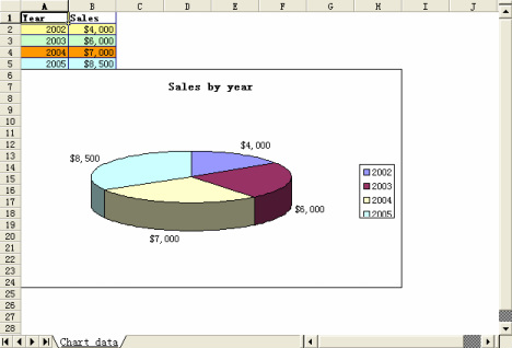
sheet.Range["A1"].Value = "Year";
sheet.Range["A2"].Value = "2002";
sheet.Range["A3"].Value = "2003";
sheet.Range["A4"].Value = "2004";
sheet.Range["A5"].Value = "2005";
//Sales
sheet.Range["B1"].Value = "Sales";
sheet.Range["B2"].NumberValue = 4000;
sheet.Range["B3"].NumberValue = 6000;
sheet.Range["B4"].NumberValue = 7000;
sheet.Range["B5"].NumberValue = 8500;
//Style
sheet.Range["A1:B1"].Style.Font.IsBold = true;
sheet.Range["A2:B2"].Style.KnownColor = ExcelColors.LightYellow;
sheet.Range["A3:B3"].Style.KnownColor = ExcelColors.LightGreen1;
sheet.Range["A4:B4"].Style.KnownColor = ExcelColors.LightOrange;
sheet.Range["A5:B5"].Style.KnownColor = ExcelColors.LightTurquoise;
//Border
sheet.Range["A1:B5"].Style.Borders[BordersLineType.EdgeTop].Color = Color.FromArgb(0, 0, 128);
sheet.Range["A1:B5"].Style.Borders[BordersLineType.EdgeTop].LineStyle = LineStyleType.Thin;
sheet.Range["A1:B5"].Style.Borders[BordersLineType.EdgeBottom].Color = Color.FromArgb(0, 0, 128);
sheet.Range["A1:B5"].Style.Borders[BordersLineType.EdgeBottom].LineStyle = LineStyleType.Thin;
sheet.Range["A1:B5"].Style.Borders[BordersLineType.EdgeLeft].Color = Color.FromArgb(0, 0, 128);
sheet.Range["A1:B5"].Style.Borders[BordersLineType.EdgeLeft].LineStyle = LineStyleType.Thin;
sheet.Range["A1:B5"].Style.Borders[BordersLineType.EdgeRight].Color = Color.FromArgb(0, 0, 128);
sheet.Range["A1:B5"].Style.Borders[BordersLineType.EdgeRight].LineStyle = LineStyleType.Thin;
//Number format
sheet.Range["B2:C5"].Style.NumberFormat = "\"$\"#,##0";
chart.PlotArea.Fill.Visible = false;
Step 4 Create Pie Chart in Excel
Now, according to the data above, we can create a pie chart in Excel worksheet and set some parameters like position and title.
//Create a chart
Chart chart = sheet.Charts.Add(ExcelChartType.Pie3D);
//Set region of chart data
chart.DataRange = sheet.Range["B2:B5"];
chart.SeriesDataFromRange = false;
//Set position of chart
chart.LeftColumn = 1;
chart.TopRow = 6;
chart.RightColumn = 9;
chart.BottomRow = 25;
//Chart title
chart.ChartTitle = "Sales by year";
chart.ChartTitleArea.IsBold = true;
chart.ChartTitleArea.Size = 12;
Step 5 Save and Preview
//Save the file
workbook.SaveToFile("Sample.xls");
//Launch the file
System.Diagnostics.Process.Start("Sample.xls");
Effective Screenshot:
With C# we can create Pie Chart in Excel without Microsoft Excel installed on system. Through the help of Spire.XLS, we can do this job effortlessly. Spire.XLS is a professiona .NET Excel component which enables developers to operate Excel file via C#/VB.NET/Silverlight.
Download Spire.XLS Here
Make sure Spire.XLS and Visual Studio are correctly installed on system. Follow the simple steps below to create pie chart in Excel.
Step 1 Create Project
Create a C# project in Visual Studio and Add Spire.Pdf.dll as reference. The default setting of Spire.Pdf.dll is placed under "C:\Program Files\e-iceblue\Spire.Pdf\Bin”. Select assembly Spire.Pdf.dll and click OK to add it to the project.
using Spire.Xls;
namespace columnchart
{
class Program
{
static void Main(string[] args)
{
}
}
}
Step 2 Create Excel Spreadsheet
We can use Spire.XLs to create an Excel spreadsheet for later usage on creating column chart.
//Create a new workbook
Workbook workbook = new Workbook();
//Initialize worksheet
Worksheet sheet = workbook.Worksheets[0];
//Set the name of the chart
sheet.Name = "Chart data";
//Set whether the grid line is visible
sheet.GridLinesVisible = false;
Step 3 Write Data in Excel Spreadsheet
Write some data into the Excel spreadsheet. To make the data with a nice appearance we can use Spire.XLS to set styles, borders and number format.
//Initialize the chart series
Spire.Xls.Charts.ChartSerie cs = chart.Series[0];
//Chart Labels resource
cs.CategoryLabels = sheet.Range["A2:A5"];
//Chart value resource
cs.Values = sheet.Range["B2:B5"];
//Set the value visible in the chart
cs.DataPoints.DefaultDataPoint.DataLabels.HasValue = true;
//Year
sheet.Range["A1"].Value = "Year";
sheet.Range["A2"].Value = "2002";
sheet.Range["A3"].Value = "2003";
sheet.Range["A4"].Value = "2004";
sheet.Range["A5"].Value = "2005";
//Sales
sheet.Range["B1"].Value = "Sales";
sheet.Range["B2"].NumberValue = 4000;
sheet.Range["B3"].NumberValue = 6000;
sheet.Range["B4"].NumberValue = 7000;
sheet.Range["B5"].NumberValue = 8500;
//Style
sheet.Range["A1:B1"].Style.Font.IsBold = true;
sheet.Range["A2:B2"].Style.KnownColor = ExcelColors.LightYellow;
sheet.Range["A3:B3"].Style.KnownColor = ExcelColors.LightGreen1;
sheet.Range["A4:B4"].Style.KnownColor = ExcelColors.LightOrange;
sheet.Range["A5:B5"].Style.KnownColor = ExcelColors.LightTurquoise;
//Border
sheet.Range["A1:B5"].Style.Borders[BordersLineType.EdgeTop].Color = Color.FromArgb(0, 0, 128);
sheet.Range["A1:B5"].Style.Borders[BordersLineType.EdgeTop].LineStyle = LineStyleType.Thin;
sheet.Range["A1:B5"].Style.Borders[BordersLineType.EdgeBottom].Color = Color.FromArgb(0, 0, 128);
sheet.Range["A1:B5"].Style.Borders[BordersLineType.EdgeBottom].LineStyle = LineStyleType.Thin;
sheet.Range["A1:B5"].Style.Borders[BordersLineType.EdgeLeft].Color = Color.FromArgb(0, 0, 128);
sheet.Range["A1:B5"].Style.Borders[BordersLineType.EdgeLeft].LineStyle = LineStyleType.Thin;
sheet.Range["A1:B5"].Style.Borders[BordersLineType.EdgeRight].Color = Color.FromArgb(0, 0, 128);
sheet.Range["A1:B5"].Style.Borders[BordersLineType.EdgeRight].LineStyle = LineStyleType.Thin;
//Number format
sheet.Range["B2:C5"].Style.NumberFormat = "\"$\"#,##0";
chart.PlotArea.Fill.Visible = false;
Step 4 Create Pie Chart in Excel
Now, according to the data above, we can create a pie chart in Excel worksheet and set some parameters like position and title.
//Create a chart
Chart chart = sheet.Charts.Add(ExcelChartType.Pie3D);
//Set region of chart data
chart.DataRange = sheet.Range["B2:B5"];
chart.SeriesDataFromRange = false;
//Set position of chart
chart.LeftColumn = 1;
chart.TopRow = 6;
chart.RightColumn = 9;
chart.BottomRow = 25;
//Chart title
chart.ChartTitle = "Sales by year";
chart.ChartTitleArea.IsBold = true;
chart.ChartTitleArea.Size = 12;
Step 5 Save and Preview
//Save the file
workbook.SaveToFile("Sample.xls");
//Launch the file
System.Diagnostics.Process.Start("Sample.xls");
Effective Screenshot:
More about Spire.XLS
Spire.XLS is a professional Excel component which enables developers/programmers to fast generate, read, write and modify Excel document for .NET and Silverlight. It supports C#, VB.NET, ASP.NET, ASP.NET MVC and Silverlight. Click to learn more...
Spire.XLS is a professional Excel component which enables developers/programmers to fast generate, read, write and modify Excel document for .NET and Silverlight. It supports C#, VB.NET, ASP.NET, ASP.NET MVC and Silverlight. Click to learn more...
 RSS Feed